FlexAFM and nanomotion sensing unveil cellular responses, offering new insights into bacterial behavior and potential ...


12.07.2024

Héctor here, your AFM expert at Nanosurf calling out for people to share their Friday afternoon experiments. Today I carry on datamining on the fridayAFM and Nanosurf databases (more than 3000 and more than 70000 images respectively).You will learn:
Datamining consists in finding patterns in large datasets.
For instance, finding that there is a correlation between how many cars someone owns and the proximity to the beach.
Historically, datamining and AFM were two terms that didn't quite match together, because regular users don't generate huge number of images. However, this is a trend that is inverting, and there are people working actively on how to apply datamining (or machine learning) techniques to AFM-based research (e.g. see Ref 1).
The turn of paradigm happened because nowadays you can obtain a big amount of AFM images in a short period of time and build collections of data relatively easy (at 10s per scan, on a typical workday of 8h one can obtain almost 3000 images).
For instance, the video of how magnetization changes in electrical steel (and the corresponding appnote), took about 700 images all captured with the same probe.
Coming back to datamining, in my case, since I have been doing fridayAFM for a while, I accumulated a decent amount of images (3271 images have been captured so far to make fridayAFM possible), so, why not trying to mine some data out of them? What information is hidden within those mountains of files?
Lucky for me, Nanosurf favours the use of Python, so our Python library (see also NSFopen) can be both used to control the AFM and to manipulate the data generated by it. So I made this script below which lets the user select a folder, automatically scan the contents of the folder looking for *.nid files, and saves the metadata of the AFM files to a CSV file. In my case, instead of dumping all the information of the header file I choose to get things like when the image was captured, the number of pixels, the scan speed, or the type of AFM used...
from NSFopen.read import nid_read
from os import listdir, walk
from os.path import isfile, join
from tkinter.filedialog import askdirectory
import re
import matplotlib.pyplot as plt
import pickle
import pandas as pd

savename='Nanosurf_S_database'

# Scans the directory selected by the user
# (using the GUI) looking for nid and nhf files
folder = askdirectory()
nidfiles = []
nhffiles = []
for dirpath, subdirs, files in os.walk(folder):
    for x in files:
        if x.endswith(".nid"):
            nidfiles.append(os.path.join(dirpath, x))
        elif x.endswith(".nhf"):
            nhffiles.append(os.path.join(dirpath, x))

######
#This can be ignored, use it only if the previous step
#was too long and want to  avoid repeating it everytime
with open(savename, "wb") as fp:   #Pickling (i.e. saving the nidfiles variable)
    pickle.dump(nidfiles, fp)

with open(savename, "rb") as fp:   # Unpickling (i.e. loading a variable from a saved file)
    nidfiles = pickle.load(fp)
######

startindex=0 #If you already processed some of the data, change this to start from where you left last time
scanranges=[]
scanpixels=[]
filesskiped=[]
scanspeed=[]
scanheadtype=[]
cantilevertype=[]
scandate=[]
opmode=[]
pgains=[]
igains=[]
dgains=[]
setpoints=[]
empytlist=[]
freqs=[]
excitation=[]
vibration=[]

#Empty data tries to save (if savefile exists, or creates it if it didn't exist).
df_empty = pd.DataFrame({'Filenames':empytlist, 'Scan Range [um]': empytlist, '# of pixels': empytlist,'Line Rate [s]':empytlist,'Scanhead':empytlist,'Cantilever Model':empytlist,'Scan date':empytlist,'Op. mode':empytlist,'P Gain':empytlist,'I Gain':empytlist,'D Gain':empytlist,'Setpoint':empytlist,'Vibration freq.':empytlist,'Excitation ampl.':empytlist,'Vibration ampl.':empytlist})
df=df_empty
file_name = savename+'.csv'
df.to_csv(file_name, index=False)


for i in range(startindex, len(nidfiles)):

    try: #Use try because there could be files with different format but same extension.
        afm = nid_read(nidfiles[i])

        param = afm.param #Parameters available
        #dir(param) To check names

        # Scan speed (Line rate in s)
        speed=param.Scan['time/line']['Value'][0]
        scanspeed.append(speed)
        # Scan Range [um]
        scansisize=param.Scan['range']['Value'][0]
        scanranges.append(float(scansisize)*1e6)
        # # of pixels
        text=param.HeaderDump['DataSet\Parameters\Imaging']['Datapoints']
        pixels=re.findall(r'\d+', text)
        scanpixels.append(int(pixels[0]))
        # ScanHeadType
        head=param.HeaderDump[r'DataSet\Calibration\Scanhead'][r'HeadTyp']
        scanheadtype.append(head)
        # Cantilever Model
        cantilever=param.HeaderDump['DataSet\DataSetInfos\Global']['Cantilever type']
        cantilevertype.append(cantilever)
        # Scan date
        date=param.HeaderDump['DataSet-Info']['Date']
        scandate.append(date)
        #Op. mode
        mode=param.HeaderDump['DataSet-Info']['Op. mode']
        opmode.append(mode)
        #PID
        pgain=param.HeaderDump['DataSet-Info']['P-Gain']
        pgains.append(pgain)
        igain=param.HeaderDump['DataSet-Info']['I-Gain']
        igains.append(igain)
        dgain=param.HeaderDump['DataSet-Info']['D-Gain']
        dgains.append(dgain)
        #Setpoint
        sp=param.HeaderDump['DataSet-Info']['Setpoint']
        setpoints.append(sp)
        #Vibration freq.
        freq=param.HeaderDump['DataSet-Info']['Vibration freq.']
        freqs.append(freq)
        #Excitation ampl.
        eampl=param.HeaderDump['DataSet\DataSetInfos\Feedback']['Excitation ampl.']
        excitation.append(eampl)
        #Vibration ampl.
        vampl=param.HeaderDump['DataSet\DataSetInfos\Feedback']['Vibration ampl.']
        vibration.append(vampl)

        #Create a dataframe to save to CSV
        df = pd.DataFrame({'Filenames':nidfiles[i], 'Scan Range [um]': scanranges, '# of pixels': scanpixels,'Line Rate [s]':scanspeed,'Scanhead':scanheadtype,'Cantilever Model':cantilevertype,'Scan date':scandate,'Op. mode':opmode,'P Gain':pgains,'I Gain':igains,'D Gain':dgains,'Setpoint':setpoints,'Vibration freq.':freqs,'Excitation ampl.':excitation,'Vibration ampl.':vibration})

    except:
        filesskiped.append(nidfiles[i])
        df = df_empty
    i=i+1
    print(str(i)+" \ " + str(len(nidfiles)))

    #Saves new data to CSV file in a new row.
    df.to_csv(file_name, mode='a', index=False, header=False)

    scanranges=[]
    scanpixels=[]
    scanspeed=[]
    scanheadtype=[]
    cantilevertype=[]
    scandate=[]
    opmode=[]
    pgains=[]
    igains=[]
    dgains=[]
    setpoints=[]
    freqs=[]
    excitation=[]
    vibration=[]
After running the script, the result is a CSV file that can be either imported back onto Python, or Excel, or any other plotting software.
Ok Ok... but what it shows?
Well, it shows for instance how many images where taken with each type of scanhead.

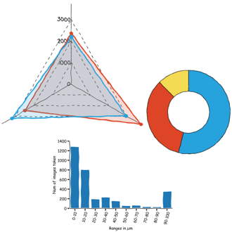
Or which scan sizes are the prefered ones when I prepare material for fridayAFM (see graph below).
It turns out that I like a lot doing small area scans and full scans, and avoid pretty much everything in between.

This likely indicates that once I have a few small scans here and there, then I tend to image the whole sample without more intermediate steps. It saves time and prevents tip degradation, because the tip only moves a lot when doing the full scan, the rest of the time only moves a small range.
Or maybe it is the result of having a button that says "Full scan range".
Speaking of probe usage... I obtained this interesting plot

Showing that the vast majority of the images I took for fridayAFM were done with the same model of probe, Tap 190, and that the second most used, is not even doing half of the images than the first one.
This tells me that probably, to get good quality statistical data, I should focus the analysis on the images taken with that probe. So, What's next?
Next, a common question I get a lot "Which gains should I use with this probe and this sample or this AFM model?" Now we can see. This is my "telemetry" compared to the Nanosurf database.
 It is rather interesting that the values are quite similar, but yet there is still room for personal variations. What does it mean this difference? Maybe if I add another parameter you will see. This is what happens when we compare average probe speed (how fast the AFM scans).

It turns out (if we assume the image quality is the same), that by having more I gain and less D gain, I'm able to scan faster.
Cool right? Feels like trying to improve the time on a race by looking at which gear is used in each corner.
Let's recap. Thanks to the Nanosurf Python interface, I was able to automate processing AFM data and performing some basic datamining on it. This lets us see things like preferred scan size, or probes used, or for instance, for one type of probe, which are the most common PID gains used. Just a sneak peek of what is possible without throwing too much data at you.
I hope you find this useful, entertaining, and try it yourselves. Please let me know if you use some of this, and as usual, if you have suggestions or requests, don't hesitate to contact me.
References:
[1] Sergei V Kalinin et al 2023 Mach. Learn.: Sci. Technol. 4 023001 DOI 10.1088/2632-2153/acccd5
23.06.2026
FlexAFM and nanomotion sensing unveil cellular responses, offering new insights into bacterial behavior and potential ...

27.05.2026
Explore Alejandro Silhanek’s innovative spintronics research, showcasing how spin waves can be investigated leveraging ...
.jpg?width=330&height=330&length=330&upsize=true&upscale=true&name=Mayfield%20Girls-202581%20(1).jpg)
19.05.2026
A group of young girls from Mayfield school wanted to start a F24 electric car racing team, and Nanosurf decided to ...

08.12.2024
Learn how to make a Python code to interface your AFM with a gamepad.
01.10.2024
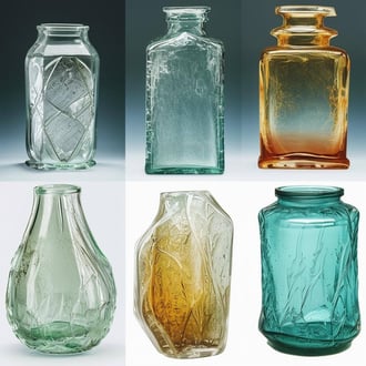
Discover how different types of glass age and degrade over time, and learn how to use AFM technology to investigate ...
11.07.2024
FridayAFM: learn how to perform datamining on large sets of AFM data.
Interested in learning more? If you have any questions, please reach out to us, and speak to an AFM expert.