Discover how Nanosurf's industrial automated AFM systems are developed from concept to delivery, ensuring precise ...

31.05.2024

Héctor here, your AFM expert at Nanosurf calling out for people to share their Friday afternoon experiments. Today I will show you how to study roughness of surfaces using Gwyddion.You will learn:
During the last few weeks I spent a lot of time inside of a clean room doing roughness measurements, so I thought it will fit to dedicate this #fridayAFM to talk about roughness and some easy experiments you can do with Gwyddion to understand it better. So lets start!
First of all, we will start by generating a test surface in Gwyddion, if you want to know more about this, probably it is a good moment to read again some previous fridayAFM's like:
1. As I was saying, we start by generating a test surface, which today will be created using ballistic deposition. This is the type of surface you will get if you are depositing a thin film, like metal films, or if you are gently oxidizing a very flat surface.

We will use a 1 by 1 μm image at 500 px.

For the particles, I choose something that gives a 100% coverage. How large the range between minimum and maximum is up to you, but I choose 1 nm particles because with standard probes this is more or less the smallest particle you can detect on a rough surface.

Hit "OK" and this will be our ideal surface.

2. Using the procedure explained on previous fridayAFMs, we generate models of probes with different apex radius.

3. Using the modeled tips and the ideal surface we simulate the result of imaging that surface with those tips.

(We did this before on the Frankenstein's monsters ).

4. Next we will simulate adding different levels of noise to the ideal surface.

You can think of this noise as coming from acoustic noise in the room, electronic noise, bad surface tracking...

The amount of noise is up to you (by changing the RMS value), I went for several different levels of noise but where I can still visually differentiate the ideal features.

This is the result.

5. Then we calculate the Power Spectrum Density (PSD).

The PSD is explained in detail on Gwyddion's documentation. Here it is sufficient to say that there are many indicators of roughness, and which one you use is up to you or your target application, but PSD is a kind of Swiss-knife tool that has a bit of everything on it. Basically it tells us how much features of different sizes contribute to the roughness of a surface.
 I used the radial PSDF Quantity because this sample is homogeneous in all directions and I'm interested in features of different sizes.

6. Export the data of the PSD to txt (right click on the graph to reveal the export menu), and then import into Excel.

After repeating the process for all the surfaces here are the results.
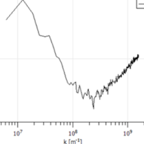
Effect of adding noise to an ideal surface.

The bottom axis is 1/nm which means that small features appear on the right and big features appear on the left. As we can see, increasing the noise amplitude increases the right side of the curve.
Effect of blunting the tip.

As the tip gets more blunted, we loose fine details, hence the right hand side of the graph decreases.
The question now, is, nothing affects the left side of the graph?
Yes, we need large features, like for instance adding waves.

You can think of these waves as the effect of vibrations because the tip moves too fast in relation to the surface, or because the feedback loop has gains too high and thus produces vibrations.

There might be other ways of simulating similar effects, but this one is quick and simple.
 So... what is the effect of the waves?
This is the effect of long range artefacts on the PSD.

What about the middle part of the PSD? This is affected by the smoothing of the features in the image, which is an effect that tends to happen when the PID feedback loop is not able to track the surface of the sample (either because gains are too low or because the scan speed is too high for the bandwidth of the probe). This is how you can simulate the effect.
7. Start with the ideal surface we created at the beginning.
 We will use SPM Modes>Force and Indentation>PID simulation

Here you can see the effect of imaging your surface with different gains on your feedback loop.

In my case, I have to lower the gains a lot and also decrease the PID/scan speed ratio, but your case could be different as these parameters can depend on the size of the features and scansize/pixel ratio.
8. Add noise to the new generated images. In my case, about 4 nm RMS seems a good value.

9. Calculate the PSD function for all the new generated surfaces and add the data to Excel as we did before.

Here are the results:
This is the effect of having bad topography tracking.
![]()
We can see how in this case the middle and right parts of the graph are the ones affected. This happens because bad PID tracking looses the small and medium features, but is still able to detect the large features (large in x y and also in z).
What happens when we add the noise?
Effect of bad tracking plus noise.
![]()
The noise increases the right hand side of the graph.
Now, why is any of this important? Why the long post about PSD?
10. Use the Statistical tool and calculate the surface roughness Sq.

This one is the most used parameter in AFM literature.

and this is how Sq looks like in the surfaces we created here.

Notice that out of all the examples, 4 result in almost the same Sq value. If we restrict ourselves to this roughness indicator alone, we will be missing information. On the PSD function on the right, we can see that compared with the ideal surface, these surfaces have either higher noise (right part, like the case of 1 nm noise and PID 15 plus 4 nm noise), additional long range features (left part, like the case with 5 nm waves), or bad surface tracking (middle part, like the case of the PID 15).
Similarities and differences between these 4 images can be seen in the images themselves.

The difference between the ideal and the ideal with 1 nm noise is minimal, here Sq was a good indicator, however, the case with 5 nm waves or the PID 15 have features that are slightly different than the ideal surface, yet their Sq value is very similar.
Let's recap. Roughness measurements are a key element to our day to day technology. From mirrors to operate lithography machines that are used to fabricate chips, to coatings that prevent food from going bad. Which roughness indicator you use depends on your application. One useful one is the Power Spectrum Distribution, and one very often used is Sq. Here, simulating surfaces, tips, noise, and bad PID tracking, we saw how different effects affect the shape of the PSD but not so much the Sq values in some of the cases. Noise raises the right hand side of the PSD function, tip blunting lowers the middle-right-handside, and long range artifacts raise the left side. Interestingly, bad PID tracking plus noise twist the graph, and if the parameters are just correct, this results in the same Sq values as the ideal surface, although the image of the surface is clearly different.
I hope you find this useful, entertaining, and try it yourselves. Please let me know if you use some of this, and as usual, if you have suggestions or requests, don't hesitate to contact me.
Further reading:
[1] ISO 21920-2:2021 Geometrical product specifications (GPS) — Surface texture.
[2] Measuring the flattest surfaces in the Universe: roughness measurements with AFM
[3] D. Nečas and P. Klapetek: One-dimensional autocorrelation and power spectrum density functions of irregular regions. Ultramicroscopy 124 (2013) 13-19, doi:10.1016/j.ultramic.2012.08.002
25.02.2026
Discover how Nanosurf's industrial automated AFM systems are developed from concept to delivery, ensuring precise ...

10.02.2026
High-end industrial solution are powered by accurate software that coordinate all their functions. Discover the ...

20.01.2026
Read how Nanosurf designs AFM stages to meet industrial challenges, ensuring precision and stability in AFM systems for ...

08.12.2024
Learn how to make a Python code to interface your AFM with a gamepad.
01.10.2024
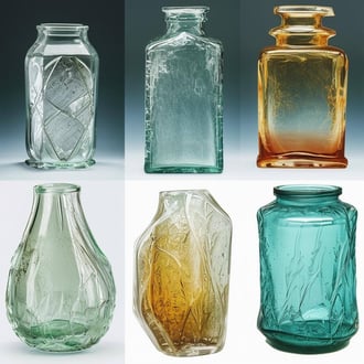
Discover how different types of glass age and degrade over time, and learn how to use AFM technology to investigate ...
11.07.2024
FridayAFM: learn how to perform datamining on large sets of AFM data.
Interested in learning more? If you have any questions, please reach out to us, and speak to an AFM expert.