Discover the capabilities of WaveMode AFM in characterizing bottlebrush polymers with unprecedented detail and speed, ...

22.12.2023

Héctor here, your AFM expert at Nanosurf calling out for people to share their Friday afternoon experiments. Today I will show you how to do some basic particle analysis with Gwyddion.
Particle detection, particle counting, template match, correlation search, are different names meaning (more or less) the same thing, identifying and quantifying things in an image. How many beads/spheres are there in this image? How many shards in the other image? What is the size distribution of the beads, what is the orientation of the shards?

I get many emails asking me to try this or try that, many end being #fridayAFM posts, I also get support questions (not always from customers, but I'm always happy to chat about AFM), and I also get requests to explain things, or to show how they could be done. Today I'm trying to fulfil one of there requests about particle counting, and since I don't regularly do it, and is kind of new to me, I categorize it as #fridayAFM, because I'm not sure how well is going to work.
So, let's see if we can play around with particle counting using Gwyddion.
1. - Lets start by creating a test image. I'll use the Synthetic tool to create a new image, and the object deposition (you can use a real AFM image if you have one and skip this step).

This is similar as when I created test images to train a neural network to "de-noise" AFM data.

In this case I'll use a 10 by 10 μm2 image with 1024 by 1024 px2. Values that are not soo off compared to what a real AFM image will look like.

The shape of the objects will be spheres, and the diameter will be approximately 200 nm, with some spread to try to imitate a real sample. The height is 100 nm, so they are a little bit compress in the vertical direction.

The last step, which is the coverage is the most critical in this example, as we want to have a few examples of spheres overlapping, but also several examples of isolated spheres. Play with the coverage value until you get something that works for you (or that resembles the images you usually get). This below is the result I obtained.

2. - The next step is to mark the objects in the image. In a case like this with only one type of objects, and flat background, Otsu works well.

You can see here the image with the mask applied.

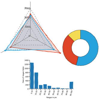
3. - With this is already posible to do some basic analisis. For instance, by going to the summary it is possible to see things like number of objects or total area covered.

And the results can be exported, for instance to be plotted in excel.

"What if we only want to select the beads of a certain size of shape? I tried the other grain selection methods and none helps."
Well, in that case, there is the correlation search. It goes something like this.
4. - First we need to select our template and we start by removing the mask by right-clicking onto the image.

Then, we cut out the image of one example of the feature we want to look for.

I'm going for one of the isolated spheres.

The detail image now includes the object and the background, so if we ask the software to look for this object (i.e. this template), it will try to find objects with a square background around, this is why I also did a mark with Otsu to mask only the sphere and forget the background.
5. - Next step is to look for the template by going to Correlation Search (remember to click on the main image to have it selected)

The menu is quite straight forward, you select the template and the threshold. I marked the "Use mask" because I want to avoid the background in the template (that is why we marked it in the step above). The correlation method is down to you, try and see which one works better, same for the threshold. For the output, we want the objects to be marked.

The new mask looks something like this:

As you can see, only the objects similar to the template are marked, and if we now open the summary, we get the values corresponding to these objects.

What else can we obtain?
6. - For instance, we can get the x and y coordinates. For that we need to go to Correlate and plot y vs x and export the graph data.

I mention x and y coordinates because those are the most familiar to me, but there are other properties such as orientation (i.e. moment). My advise here is to look at the literature in your field and see which properties might be of interest.

One little thing. Once you have the graph, to export simply right click on the graph and export as CSV for instance.
Ok, this is nice, but... what if we have more than one species in the sample. For instance, spheres and shards.
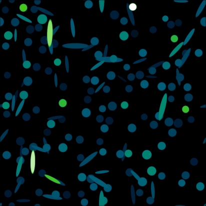
7. - To create an image that has two different objects, we start by generating the shards image. We will use the spheres parameters, but just change the shape and orientation parameters until the spheres look like shards.

The orientation parameter is on the other tab. Change the spread in the orientation to obtain random alignment of the shards.

The result is something like this.
 8. - If we want to use the template from the other example. How can we import it? Well, if you saved the other example as *.gwy (Gwyddion) format, then just open the file, and grab the template from the data browser onto the shards image. This will copy the template from one file onto the other.

This is really useful if you have a very good image of the template but you image in separate days or have measurements from different instruments.
Ok, but how we generate the test picture? When doing the object deposition, there is an option that lets you start from the current frame. By selecting it we can add a second type of objects to an existing image.

The result is something like this. Note that you can use this also with actual images taken with your AFM to see how depositing different objects might look like over your surface.

The rest of the process is the same, correlation search, select the template...
9. - One important step is to have the same pixel size (also, the total number of pixels in the template should be less than in the image you are analyzing). To change that you can go to basic operation resampling.

You just ask to match the pixel size of the main image. This is quite critical and can led to a lot of frustration, because pixel mismatch is not something obvious.

You can experiment with the type of interpolation if the image distorts (we saw how important it could be when we show how to use machine learning to achieve Super Resolution), but for this example linear is good enough.
10. - So... once we have the right pixel size, it is just a matter of applying again the correlation search to find the beads within the shards.

Note that due to the size spread in the yize of the beads, some are too small or too large to match the template, that is likely why there are not marked.
Can we now do the oposite and mark the shards?
This is more complicated because of the asymmetry. The reason is that this search method doesn't try rotating the template, and thus cannot account for when the object is rotated in relation with the template.

At this point there are several solutions. We can for instance create several copies of the template and rotate each by small amount, so we end with lots of templates one for each angular orientation... or we can try with other software. Note that Gwyddion tutorial ends here, the next part is just to hint you how a process similar to this could be done in Python.
For this next section we will try OpenCV, which is a Python library dedicated to computer vision.

I will start from the example shown in this tutorial and modify it slightly for our needs.
First I will save the image and the template.

Then this is the code I have.
import cv2 as cv
import imutils
import numpy as np
from matplotlib import pyplot as plt
from pathlib import Path
import tkinter as tk
from tkinter import filedialog


#GUI to select the main image and the template
root = tk.Tk()
root.withdraw()

#Load the main image and convert it to grayscale and then to edges
filename = filedialog.askopenfilename()
name=Path(filename).stem
folder=Path(filename)
img_rgb = cv.imread(filename)
img_rgb_initial = img_rgb.copy()
img_gray=cv.cvtColor(img_rgb, cv.COLOR_BGR2GRAY)
img_gray_edges = cv.Canny(img_gray,1,50)

#Load the template image and convert it to grayscale
filename2 = filedialog.askopenfilename()
name2=Path(filename).stem
folder2=Path(filename)
template_grey = cv.imread(filename2, cv.IMREAD_GRAYSCALE)#This is to show an alternative way of converting to grayscale
template_edges = cv.Canny(template_grey,1,50)

#We rotate the template up to 180 deg in as many steps as indicated by max range
maxrange=1000
for k in range(0,maxrange):
    rotated_template_edges = imutils.rotate_bound(template_edges, 180/maxrange*k)
    w, h = rotated_template_edges.shape[::-1]
    #This calculates the correlation matrix between the main image and the template.
    #Other available methods to try: cv.TM_CCOEFF  cv.TM_CCOEFF_NORMED  cv.TM_CCORR
    # cv.TM_CCORR_NORMED  cv.TM_SQDIFF  cv.TM_SQDIFF_NORMED
    res = cv.matchTemplate(img_gray_edges,rotated_template_edges,cv.TM_CCOEFF_NORMED)
    threshold = 0.25
    #We find the areas where the correlation exceeds the threshold
    loc = np.where( res >= threshold)
    #Paint squares in the main image where the correlation was high enough
    for pt in zip(*loc[::-1]):
        cv.rectangle(img_rgb, pt, (pt[0] + w, pt[1] + h), (0,255,255), 2)

#As a summary, display the different images used
plt.subplot(231),plt.imshow(img_gray_edges[:,::-1])#cmap = 'gray'
plt.subplot(232),plt.imshow(rotated_template_edges[:,::-1])#cmap = 'gray'
plt.subplot(233),plt.imshow(img_rgb_initial[:,::-1])#cmap = 'gray'
plt.subplot(234),plt.imshow(img_gray[:,::-1])#cmap = 'gray
plt.subplot(235),plt.imshow(template_grey[:,::-1])#cmap = 'gray'
plt.subplot(236),plt.imshow(img_rgb[:,::-1])#cmap = 'gray'

#Saves the result
cv.imwrite('res.png',img_rgb)
Basically what it does is convert the images to grayscale, detect edges, and then correlate the edge images trying the template at 1000 different orientation between 0 and 180 degrees.
The output of the script looks like the image below.

It might need some tweaking of the parameters, but it manages to identify some of the shards similar to the template, and illustrates the concepts.
Let's recap. We have seen how to use masks and grain detection in Gwyddion to perform statistical work on AFM images. In particular, we have seen how to use templates to detect features. This last thing was also demonstrated using the Python library openCV.
I hope you find this useful, entertaining, and try it yourselves. Please let me know if you use some of this, and as usual, if you have suggestions or requests, don't hesitate to contact me.
28.10.2025
Discover the capabilities of WaveMode AFM in characterizing bottlebrush polymers with unprecedented detail and speed, ...

27.10.2025
Read this blog and discover advanced alloy engineering and cutting-edge AFM techniques for high-resolution, ...

14.10.2025
Discover how WaveMode technology resolves the tobacco mosaic virus structure under physiological conditions with ...

08.12.2024
Learn how to make a Python code to interface your AFM with a gamepad.
01.10.2024
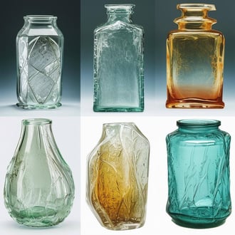
Discover how different types of glass age and degrade over time, and learn how to use AFM technology to investigate ...
11.07.2024
FridayAFM: learn how to perform datamining on large sets of AFM data.
Interested in learning more? If you have any questions, please reach out to us, and speak to an AFM expert.