Explore Alejandro Silhanek’s innovative spintronics research, showcasing how spin waves can be investigated leveraging ...

05.07.2024

Héctor here, your AFM expert at Nanosurf calling out for people to share their Friday afternoon experiments. Today I upload a brief tutorial on how to automatize roughness analysis using MountainsSPIP.You will learn:
After the post about roughness of ball point pens, many people approached me last week and asked if data analysis with MountainsSPIP can be automatize somehow, because they have to repeat the same analysis over and over but they are not very familiar with the software.
Do not panic.
Here are three ways of automatizing roughness analysis with MountainsSPIP. (Steps 1 to 6 are to setup the scene, and steps 7 and beyond are to show you how to automatize steps 1 to 6).
1. Our test data will be the surfaces we generated in Gwyddion for the roughness analysis tutorial posted a few weeks ago.

With one addition, I will add a surface with large curvature, something similar to the ball of the ball point pen. I created it in the same way as I created the other artificial surfaces in Gwyddion, this one uses waves in x and y and very low spatial frequency.

If you missed how to generate surfaces on Gwyddion, I covered that in several posts:
FridayAFM - Particle detection
FridayAFM - Neural networks and Gwyddion
2. Load data onto MountainsSPIP by drag and drop. Data in MountainsSPIP is called studiable.

The software will automatically represent the image if it is the first studiable on the project.

3. Before we begin the roughness analysis, we need to substract the large background. To do so, we are going to apply a filter that separates the roughness (small features), from the wavines (large features).

4. Adjust the cut-off depending on the size of your features to separate what you consider roughness and what is for you part of the wavines.

This will give you two new surfaces.

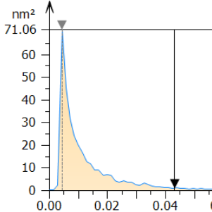
5. Now calculate the power spectrum density function of each image.

This will give you three graphs which are quite interesting.

By the way, do you know that MountainsSPIP has sticky notes which let you add fridayAFM style to your reports...

Note that I also changed the zoom factor to better show you the graphs.
As I was saying, these graphs are quite interesting and complement the discussion we were having on the post FridayAFM - Gwyddion roughness analysis. Note that Gwyddion plots the inverse of the distance so the graphs are inverted in respect to the ones on Gwyddion. Now, focus your attention on the PSD of the original surface. It looks like the ones we analyzed in Gwyddion, one "smooth" bump. Meanwhile, the one that is pure background tends to have most of its contribution towards high values of x, while the one that is "roughness" has the contributions towards low values of x. Note also that the surfaces that came from the filter tend to have spikes and distances where there isn't contributions at all. This is a typical feature of filters, and can help identify when data has been filtered (e.g. to make it look better). Cool feature right?
6. With the roughness selected, click on calculate parameters, this will let you calculate roughness indicators.

This opens a menu that lets you select which standard and which indicators you want to use (I leave in default, it is not important here what you choose for this example).

After closing the dialog, you will obtain a table with the results.

Save the document.
Now we are ready to automatize all these steps.
7. The first way of automatize this roughness analysis consists in dragging a new data file which replaces the current studiable with a new one.

Automatically the analysis is redone with the new data.

8. The second automatization route consists in creating a minidoc. Select the studiable and all the steps on the workflow (also the sticky notes on the the main window) and click Save as Minidoc.

Give it some meaningful name and maybe an icon.

Believe me, it pays of spending time on the name and the icon, otherwise overtime you will forget if it was Roughness, Roughness Final, Roughness Final Final, or Roughness Extra. For instance, I have a cat to analyze steel.

After you finishing name it, you will be presented with the minidoc to fine tune it. If you don't have anything else to add, simply close it and now it is ready to be used.

9. To use the minidoc, load another estudiable into the workflow.

Then selected it, go to minidocs, and click on your minidoc.

You will see that automatically the same steps are applied to the new studiable.

So far good, this saves some time... Hold on, the last way of automatize things will blow your mind.
10. Remember that you saved the document at the end of step 6? Now go to file "apply template".

The menu that opens basically lets you choose a number of files that will be used as the studiable in the document you use as a template, and you can choose if the output is new MountainsSPIP files, images... or an excel

and like that, in seconds...

All your data files analized and reports created.

and what is better, if you are systematically studying how a parameter gets affected by some variable... the summary in CSV format which can be imported for instance into Excel.

Let's recap. We used some test images to show some of the automatization capabilities in MountainsSPIP. The automatization is particularly useful when analyzing the same type of data all the time (e.g. roughness analysis). The three methods we saw where: replace studiable; create a minidoc; save the project and use it as a template for any number of files.
I hope you find this useful, entertaining, and try it yourselves. Please let me know if you use some of this, and as usual, if you have suggestions or requests, don't hesitate to contact me.
Extra:
When a PSD is selected, you get a new menu, and among the things you can do, you can export the results, in case you want to plot them somewhere else.

27.05.2026
Explore Alejandro Silhanek’s innovative spintronics research, showcasing how spin waves can be investigated leveraging ...
.jpg?width=330&height=330&length=330&upsize=true&upscale=true&name=Mayfield%20Girls-202581%20(1).jpg)
19.05.2026
A group of young girls from Mayfield school wanted to start a F24 electric car racing team, and Nanosurf decided to ...

27.04.2026
Explore cutting-edge research at IEMN with DriveAFM systems for advanced nanotechnology and microfabrication, enhancing ...

08.12.2024
Learn how to make a Python code to interface your AFM with a gamepad.
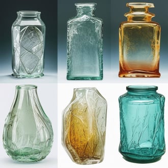
01.10.2024
Discover how different types of glass age and degrade over time, and learn how to use AFM technology to investigate ...
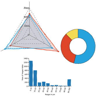
11.07.2024
FridayAFM: learn how to perform datamining on large sets of AFM data.
Interested in learning more? If you have any questions, please reach out to us, and speak to an AFM expert.